Most powerful yet unsung Excel functions for Compensation professionals

I thought about writing a more technical post but didn’t know where to start from.
It could be a nice series of post starting from scratch, however after some googling, I thought it might be more beneficial to write about the unknown and/or unrecognized magic words that saves your time in front of the screen covered with cells.

As I advance in my career in Rewards area, I started to use macros more and more. This could be a good subject for another post but there are some formulas or that saved my life.

I will list some of these Excel functions and give you examples how and when to use it. You will not find the generic VLOOKUP() and similar essential formulas in the following list. Here we go:

INDEX() and MATCH() combination

Slowly leave your VLOOKUP() down and kick it to me. Nobody needs to get hurt!

Yes, this is it. The combination of INDEX and MATCH is one of the most powerful formula combination to save your life while trying to extract data from a data table with multiple input variables.

Let’s say we have a table like the one below and we would like to get the “Benefit” amount of the employee with the ID of “EMP3”:

The formula would look like this:

=INDEX(C4:E13,MATCH(“EMP3”,B4:B13,0),MATCH(“Benefit”,C3:E3,0))

As you can see, the index formula is the main formula where you need to identify as a first variable the area where the values are stored. You should not choose the left and top column in this area hence they are identifier row and column which will help us in the second and third variable.

INDEX() function works this way: I will give you the row number and column number and the cell at the intersection of those is the value I want.

MATCH() function a little bit different: Give me the exact place of this value in a range/series.

So with the MATCH() functions we identify the row and column numbers that INDEX() want. We want the row number of EMP3 in unique ID’s and the type of the pay “Benefit”.

IFERROR()

Life cannot be without errors. More important thing is how you handle the errors. This formula can give you a better control in your data management if used properly.

Let’s say, you want to pay 5,000 USD even there’s an error in the calculation (in this example addition of three cells) of a cell.  Normally, the formula would look like this:

=A1+F45+K7

What if K7’s value is not a number? The Excel would give you an error for sure. To avoid seeing “#….!”, you can use IFERROR() and tell that even if there’s an error my sum would be 5,000:

=IFERROR(A1+F45+K7,5000)

Pretty simple, huh?

AND() and OR()

The basic logical operators are here. If you want to check two conditions that they are TRUE at the same time (AND) or at least one of them (OR) you can use these:

=AND(“Arif” = “Arif”, “Excel” = “Excel”)

will always give you a boolean result of TRUE like

=OR(“Cat” = “Dog”, (3-2) = 1)

does.

Now, before going forward I would like to warn you about the following two functions. Although they are saving lives in some instances, they are called as “volatile functions”.
A Volatile Function is one that causes recalculation of the formula in the cell where it resides every time Excel recalculates. This occurs regardless of whether the precedent data and formulas on which the formula depends have changed, or whether the formula also contains non-volatile functions. That’s why you have to be really careful and mostly avoid using this.

OFFSET()

We will use the same table above. As per that data table, we will analyze the below formula and see how OFFSET() function works:

=SUM(OFFSET(C4,4,1,3,2))

Translation is: We will start from C4, go 4 cells down, then 1 cell right and starting from that cell we take all 6 values in a 3×2 table and add them all… Makes sense, right?

The table is this part:

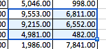
So, the result would be in this case 37,594 in case you want to try.

INDIRECT()

I use this mostly in consolidation of various files with pre-set names that can be linked to an identified variable.
For example, you have one template for each country in your region and you want to get a value from its first sheet, cell A1:

It might be confusing, but the above figure is pretty self-explanatory. Please note that, you will see a #REF! error, if the target Excel file is not open.

I will continue to explain other functions in the Part II of this post and hope that this will help you come up with a better Compensation analyses!